This document will guide the user through a basic whole-pattern decomposition of a single phase using the Pawley method. This method is simpler than the Rietveld method and will provide a closer fit, however the the refined parameters are not physically meaningful so the amount of information obtained is limited. In this tutorial, I will refine a corundum scan taken on our Bruker D8 Discover ("Alice").
The diffractogram can be downloaded in .xye format. You may also want to look at the finished GSAS-II project.
Installation
Visit the GSAS-II website and follow the installation instructions for your platform (GNU/Linux, Windows, MacOS). Arch Linux users can install gsas2-svn from the arch user repository. Upon running GSAS-II for the first time, you should see a terminal window and several empty windows, similar to the screen shot below.
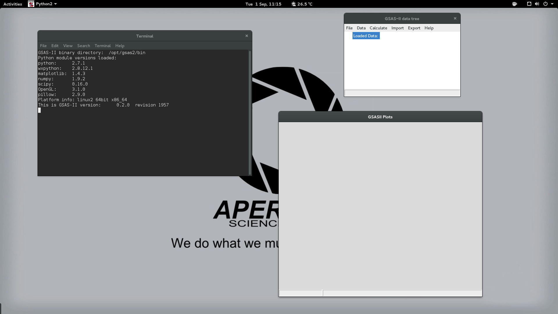
The terminal window is not normally used, though it can provide useful information if your refinement is not succeeding. The other two windows are the plotting window and the data tree window. They are currently empty since we have not yet imported any data.
Load Powder Data
First we must load a powder data file to refine against. First, export your data from Eva as a .xye file. In the data tree window, select . The first dialog to appear will ask you to choose the file containing the powder diffraction data. The second dialog asks for an instrument parameter file. If you do not have an instrument file, click Cancel and you are prompted to choose a generic instrument (eg. CuKα). You should now see your data listed in the data tree window.
Create Phase Object(s)
The next step is to create a phase object that can be refined against the powder data. There are two options for this: importing a .cif file or creating a blank phase. Once the phase has been created you should see an entry for it in the data tree window (you may have to expand the Phases entry.
Importing a Phase from a .cif File
If a .cif file is available for your material, this is the easier option. The materials project may have one you can download for your material. To import a .cif file, in the data tree window select the menu . You will be asked to associate this phase with one of more previously imported data ("histogram"); you can select your powder data, or wait to do so in the next section.
Creating a Blank Phase
In the data tree window, select the menu Data → Add phase, you will be prompted to name the phase.
Prepare for First Refinement
Before running the first refinement cycle, it's necessary to set some initial values. If you imported a .cif file, some of these may already be set for you. This section assumes you have created a blank phase.
In the data-tree window select your phase from the Phases list. A new data display window should appear. Select the Data tab. Enter your space group in appropriate text box. GSAS-II requires spacegroup terms to be separated by a space. The corundum spacegroup (R-3c) is entered as "R -3 c". Press enter and confirm your choice. You will now notice that your choices for unit-cell parameters are restricted to a and c due to the crystal system associated with this spacegroup. Enter approximate unit-cell parameters in the appropriate textboxes. Wikipedia lists a=4.75Å and c=12.982Å for corundum so let's start there. Farther down you will find a section labeled Pawley controls. Check the checkbox labeled Do Pawley Refinement.
Next switch to the Data tab. If you see a message reading ``This phase has no associated data'', you will first need to create a histogram by selecting the menu Edit → Add powder histograms. In the new dialog, select your powder data and click okay (skip this step if you associated your data when importing a .cif file). Leave the values in this tab at their defaults for now; we will come back to them later.
We will now move to the Pawley Reflections tab. Select the menu entry to automatically create a list of reflections and to have GSAS set initial reflection intensities. The refine column contains check boxes that indicate which reflection intensities will be refined. Click on the column heading to select them all and type "y" to check them.
Lastly, go back to the data-tree and under your powder data entry, select the Sample parameters entry. In the data-display dialog, uncheck the Histogram scale factor box. If checked, GSAS will refine the intensities of the reflections as a whole, which is unnecessary since we are already refining them individually.
Evaluating Initial Fit
You are now ready to run the initial refinement. In the data-tree window, select the menu (you will be prompted to save if you have not done so yet). Assuming the refinement runs smoothly, you should be presented with a dialog asking you to Load new result? (click Yes). Click on the powder data entry in the data-tree and inspect the results in the plotting window. You may have to select the Powder Patterns tab. You should see several overlayed plots showing the original diffractogram, the calculated diffractogram, the background fit and the difference between the observed and calculated diffractograms.
Chances are, your refinement is not very good at this point, but maybe it's good enough. Use the zoom button along the bottom to view several peaks close up. Along the center of the plot you will see small vertical lines representing the predicted reflections. Hopefully, your unit cell parameters are at least close enough that the predicted reflections fall somewhere within most of the peaks. If not, you may have to manually adjust the cell parameters until you're close. Something like the figure at the right should work. Select your phase and go to the General tab, check Refine unit cell. Also, for your powder data, open the Sample Parameters dialog. Change the diffractometer type to Bragg-Brentano and enable refinement of Sample displacement. This will help correct any errors due to the sample not being mounted at the exact instrument center. Now run the refinement again. You may have to re-select your powder data in the data-tree to refresh the plot.
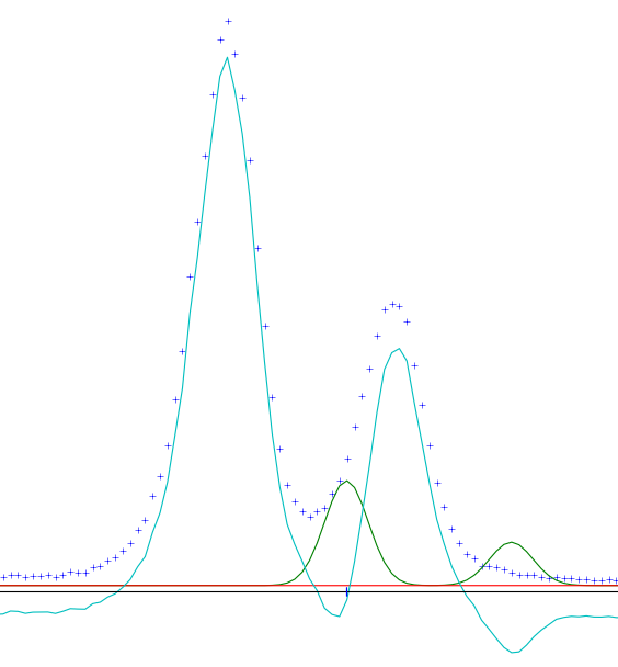
Refinement after first pass. Shown are observed (blue), calculated (green), background (red) and difference (teal).
Refining Background
Zoom out on the plot by clicking the home button and look at how well the refinement is accounting for the background. It may be helpful to zoom vertically to get a better look. In the data-tree select the Background dialog. The default is to refine three coefficients, change this to something higher if you feel the background is not fit well. For corundum I chose 10. Re-run the refinement, if you're happy with how the background looks, you can move on.
Refining Peak Width and Shape
There are two sources of line broadening in diffraction data: instrument effects and sample effects. Instrument effects are not usually of scientific interest and are lumped together and described by parameters in the Instrument Parameters section. If you used an accurate instrument parameters file, these should not need much adjusting.
Of more interest are the sample effects. These can be found in the dialog for each phase, under the Data tab. They do not have directly refineable parameters, instead you must choose a model to describe the peak shapes and widths. Since we are doing profile fitting, the parameters in this tab do not reflect their real world analogs; for that a thorough Rietveld treatment is necessary. Select whichever model you prefer and check the corresponding box. For corundum, I used size. Sample parameters are usually described well by Lorentzian functions, but the Lorentzian/Gaussian ratio can be refined by the corresponding LGMix parameter. 1 is entirely Lorentzian.
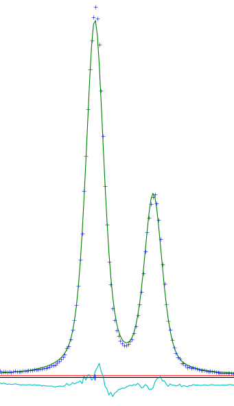
Fit after multiple refinements.
From here, continue going until you achieve the desired fit. Each time you run the Refine command, GSAS-II performs three refinement cycles. Just because the process ends does not mean that it has found the best fit. You may need to run the Refine command several times, until the calculated patterns are constant from one refinement to the next. For the corundum example, I ended with a cell parameters of 4.75903Å and 12.99294Å.